Plot elevation data (GDEM -SRTM) as contours in ggplot2

• Create an account on the Nasa earthdata website to be able to download the data.
• Go on the map view to search data and select a region.
• Search in the filter box “GDEM”.
• Select what you want, SRTM or GDEM, up to you to test.
• Download all.
• Download 1 by 1 or use the download script (.sh) you will need your username and password. For the last you would need wsl (bash or ubuntu) if you are on windows. The script file should not contain “\r”. Run it with `./yourscript.sh”.

BUT they are other ways to download it even via R:

Let them all in one folder

GDAL

From this source it is possible to merge rapidly the tif without R (faster than R). You have to use GDAL. Could be install via apt-get.

You will have to combine them in vrt and finally convert them into tif. Here I add from ASTER GDEM V003 2 files per tile (dem and num) and use only 1 the dem.

all=$(find *dem.tif)
# could also just use *tif, adapt to your needs
gdalbuildvrt mosaic.vrt $all
gdal_translate mosaic.vrt MOSAIC.tif

R

Now you have one tif for all.

Let’s load some functions and packages

library(data.table)
library(ggplot2)
library(rayshaderanimate)
theme_set(theme_bw())

zoomman <- function(loc, zoom) {
  lon_span <- 360 / 2^zoom
  lat_span <- 180 / 2^zoom
  lon_bounds <- c(loc[1] - lon_span / 2, loc[1] + lon_span / 2)
  lat_bounds <- c(loc[2] - lat_span / 2, loc[2] + lat_span / 2)
  return(data.table(lon=lon_bounds, lat=lat_bounds))
  # source: # https://www.r-bloggers.com/2019/04/zooming-in-on-maps-with-sf-and-ggplot2/
}

get.contour <- function(raster.file, level.u = 100) {
  # use in ggplot contour
  r <- raster(raster.file)
  rrc <- rasterToContour(r,  level=seq(0, 5000, level.u))
  rrc2 <- st_as_sf(rrc)
  rrc3 <- data.table(st_coordinates(rrc2))
  rrc3[, group := paste0(L1, "-", L2)]
  return(rrc3)
}

Now let’s run it

# choose your til file and the level of detail of the contour lines (here 100m)
rr3 <- get.contour('C:/Users/doria/Downloads/Outdoor/GDEM/nasa_test_02.tif', 100)

world <- data.table(map_data("world"))

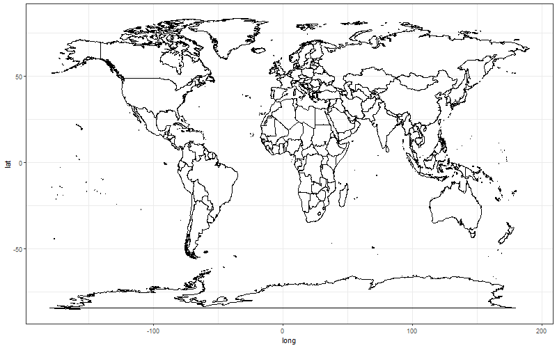
# plot the world
a <- ggplot()+
  geom_polygon(data=world, aes(long, lat, group = group),color = "black", fill=NA)
a

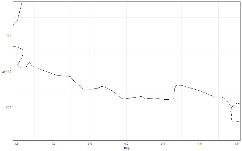
Let’s zoom in

# get your zoom center one 1 point
point.choosen <- c(0,43)


# let's create a sort of bbox by specifyng the zoom (here 7)
zoom.choosen <- zoomman(point.choosen, 7)

b <- a + coord_cartesian(xlim = zoom.choosen$lon, ylim = zoom.choosen$lat)
b

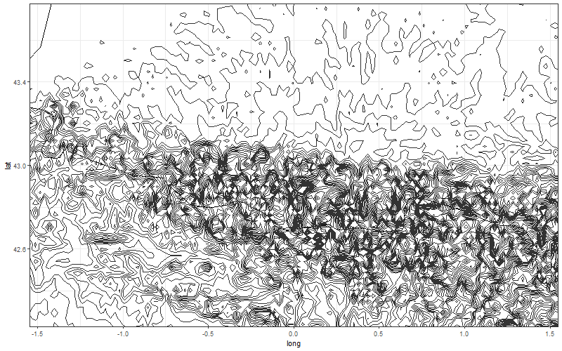
c <- b + geom_path(data = rr3, aes(x = X, y = Y, group=group), color = "grey20")
c

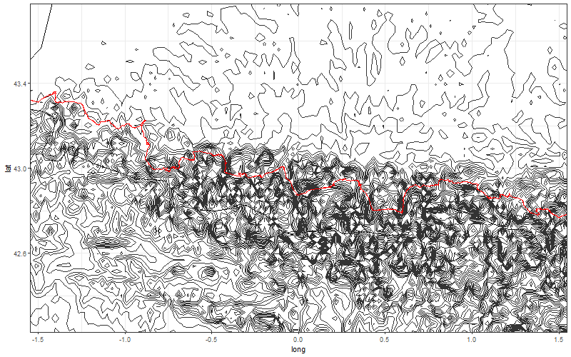
Plot a gpx

datagpx <- data.table(get_table_from_gpx("C:/Users/doria/Downloads/Outdoor/Gpx/BikeTrip2022b.gpx"))
d <- c + geom_path(data = datagpx, aes(lon, lat), color = "red")
d

Then you can do cool stuff like :

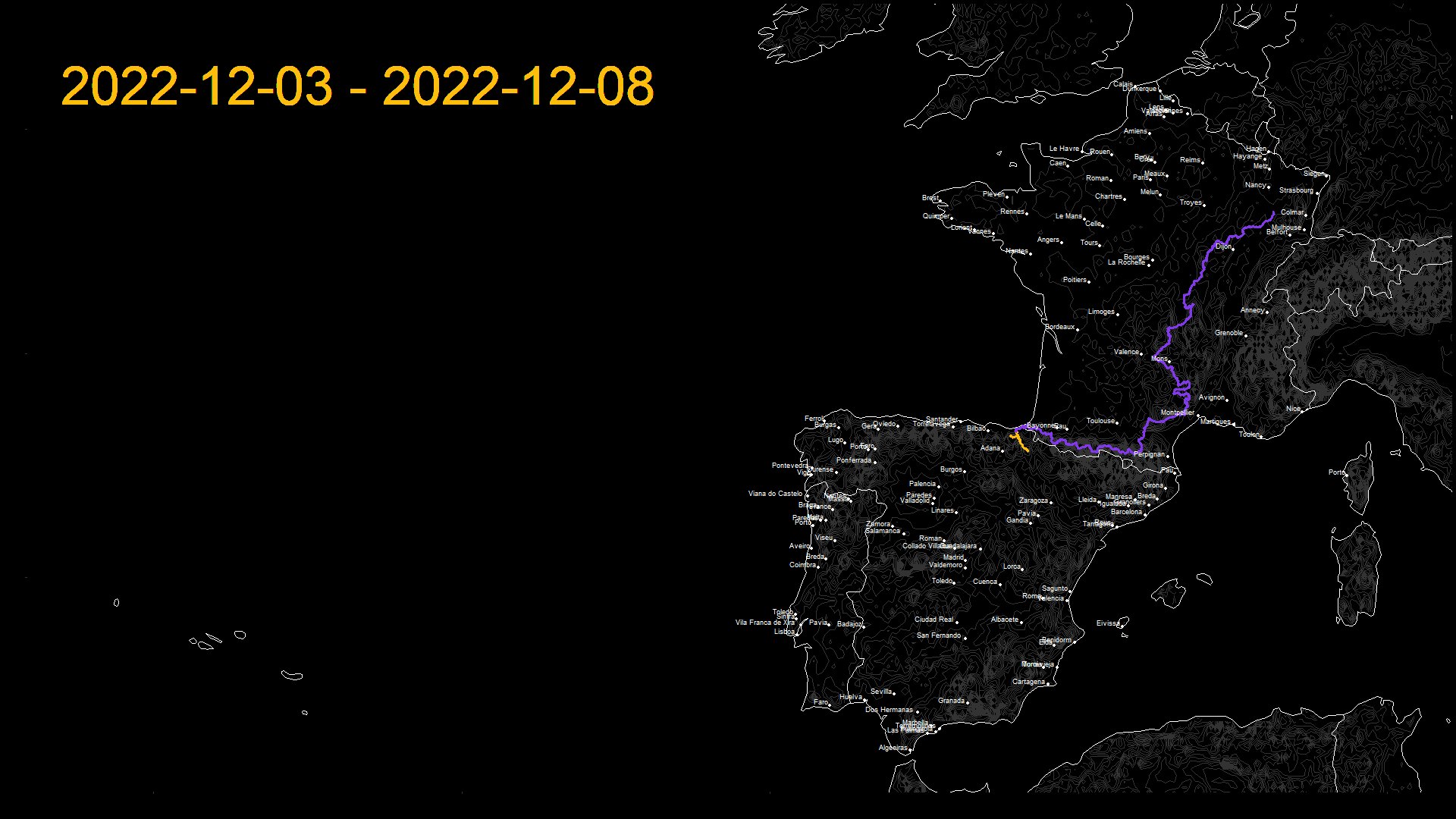
Here is the theme I used for this.

theme_set(theme_void())
theme_set(theme(plot.background = element_rect(fill = "black"),
                panel.background = element_rect(fill="black"),
                panel.grid.major = element_line(color = 'black'),
                panel.grid.minor = element_line(color = 'black'),
                axis.text=element_text(color="black")))

or even animate it with gganimate or create mp4, a lot is possible.